Ngspice varies from popular spice simulator counterparts by being fully open source and having a builtin discrete event simulator (DES) which is based on Xspice simulator [1].
DES
Simulators lets us calculate and visualize the behavior of a physical system without actually build and running it. This requires constructing a mathematical model of the physical system in which the system state is kept in a vector of numbers. Starting from an initial state and time, the simulator calculates the value of state vector for the next time step. This is continued until an end time is reached.
Continuous time simulation represents the behavior of physical systems very closely. Time steps are dynamically decreased during the simulation to capture fast events (much accurate simulation of natural physical events).
Discrete time simulations iterates the state variables at fixed time steps.
Discrete event systems iterates the state variables when an event occurs (more efficient to simulate man-made events).
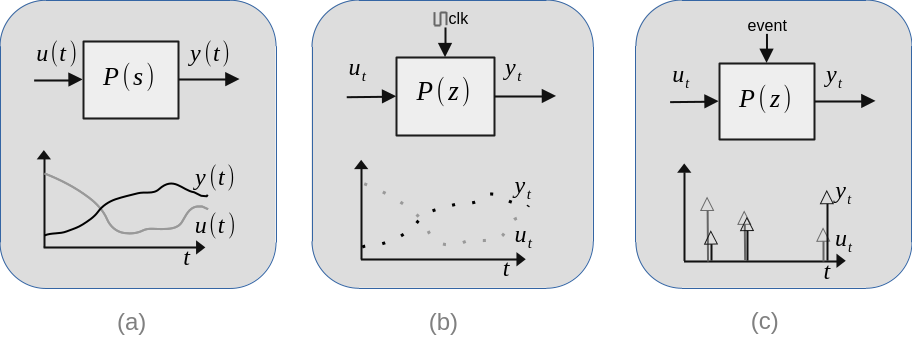
Besides, it can be said that DES covers discrete time systems since a periodic clock input can be considered as an event.
Xspice code-models
The development of Xspice was started a early 90s to make SPICE systems support board-level circuits and more efficiently simulate ICs [1]. SPICE simulators are focused on continuous time simulation of physical components by using mathematical definitions of their voltage/current relationships.
Xspice adds high level models such as limiters, comparators, mathematical operations, FIR filters, etc. Furthermore, Xspice introduces a code-model approach to define these high level operations. Xspice's code-model syntax is based on C language. It adds some special macros to access model configuration, input/output signals. Since, these macros can not be compiled by C preprocessor, Xspice passes code-models from a specialized preprocessor to generate the actual C language code file.
A new model can be defined by writing an interface specification file and C code file which implements the model behavior.
An example
This example demonstrates how to extend Xspice by new code-models by implementing a matrix gain model. Basically, it multiplies the input vector by a matrix and writes the results to an output vector. Such a model can be used in place of gain and summation blocks.
Xspice models are defined by two main files:
- Interface specification file (.ifs extension)
- C code file (.mod extension).
You can find the source files for this example in this fork of Ngspice repository. Some fragments of the code are explained below.
Interface specification file
A model is defined by its input, output and parameters. The specification file is the place to define them in plain text.
NAME_TABLE:
Spice_Model_Name:      real_mtx_gain
C_Function_Name:       ev_real_mtx_gain
Description:           "Matrix gain."
In '.ifs' format, NAME_TABLE is the block where model name and description are defined. Also, the model function's name in C code file must be declared here. Simulator will call this function many times during a simulation.
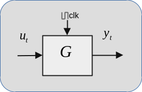
PORT_TABLE:
Port_Name:             in         clk          out
Description:           "input"    "input"      "output"
Direction:             in         in           out
Default_Type:          real       D            real
Allowed_Types:         [real]     [D]          [real]
Vector:                yes        no           yes
Vector_Bounds:         [1 -]      -            [1 -]
Null_Allowed:          no         no           no
Second text block defines the ports. It has input (in), output (out) and clock (clk) ports as shown in the diagram above. Input and output are real vector type. Clock is a scalar and it is digital (D). The aim of having a clock input is to synchronize the calculation of new output from input with the other components in the simulation. Because, Ngspice can call model's C function at any simulation time. It is model developers duty to adjust calculation time precisely. As it will be seen in the C code, output is update only at the rising edge of clock input.
PARAMETER_TABLE:
Parameter_Name:        g
Description:           "List of matrix entries of gain in row-major format"
Data_Type:             real
Default_Value:         0.0
Limits:                -
Vector:                yes
Vector_Bounds:         [1 -]
Null_Allowed:          no
PARAMETER_TABLE:
Parameter_Name:        delay
Description:           "output delay (must be greater than 0)"
Data_Type:             real
Default_Value:         1e-9
Limits:                [1e-15 -]
Vector:                no
Vector_Bounds:         -
Null_Allowed:          yes
Parameter g is a long list of numbers which holds the entries of gain matrix in row-major order. For example, the matrix
$$ G= \begin{bmatrix} 0.1 & -1 \\ 0 & 2 \\ 1 & 0.05 \end{bmatrix} $$
can be defined by g = [0.1 -1 0 2 1 5e-2].
The last parameter is delay, it is placed to get rid of a simulator warning and has not effect on the output when it is chosen to be much smaller than the simulation step size.
STATIC_VAR_TABLE:
Static_Var_Name:       state
Description:           "Data structure which keeps model's internal state"
Data_Type:             pointer
Lastly, there is a static variable created for each instance of the model that keeps the state between each call of the model function. This is defined as pointer type and it is developers duty to allocate and free the data structures pointed by this variable at the beginning and end of the simulation.
The C function file
Ngspice call model's C language function repeatedly at distinct time instants during the simulation. Time steps are calculated dynamically depending of the whole structure of the simulation. Maximum time step is provided in the simulation code, but actual time steps are decided by the simulator.
void ev_real_mtx_gain(ARGS)
{
    double      *in;          /* Values of inputs to model */
    double      *out;
    uint        n, m;
    ...
}
This is the definition of model's C function. As it can be seen, there is a special argument named ARGS. This keyword is processed by the mentioned xspice preprocessor and converted to the lines below:
void ev_real_mtx_gain(Mif_Private_t *mif_private)
{
    double      *in;          /* Values of inputs to model */
    double      *out;
    ...
}
It is converted to a xspice structure which keeps pointers to input, output and parameters.
    ...

    if(INIT) {
        cm_event_alloc(CLK_STATE, sizeof(Digital_State_t));
        clk = (void *) cm_event_get_ptr(CLK_STATE, 0);
        old_clk = clk;
        *clk = INPUT_STATE(clk);
        CALLBACK = ev_real_mtx_gain_callback;
        state = (MTXGainState *) (STATIC_VAR(state) = calloc(1, sizeof(MTXGainState)));
        if (!state)
            goto error;
        state->y = (double *) calloc(m, sizeof(double));
        if (!state->tmp)
            goto error;
    }
    else {
        clk = (void *) cm_event_get_ptr(CLK_STATE, 0);
        old_clk = (void *) cm_event_get_ptr(CLK_STATE, 1);
        state = (DLTIState *) STATIC_VAR(state);
        if (!state)
            goto error;
        if (!state->y)
            goto error;
    }
    ...
In the lines above, the logic at initialization is implemented. If INIT is true, variables which keeps a global state are allocated and initialized. And, an event callback function ev_real_mtx_gain_callback is defined. This callback function is called at some simulator events. For example, the allocated variables are freed at MIF_CB_DESTROY event which occurs at the end of simulation.
If INIT is false, clock event is saved to old clock for comparing them to detect clock rising edges. Besides, INIT is true only at the beginning of the simulation when the model's C function is called the first time.
    if (ANALYSIS == TRANSIENT) {

        ...

    }
This code-model implements only the transient simulation which operates on time axis. However, Ngspice supports AC and DC analysis. The model's behavior in other type of analysis must be implemented separately in the model's C function.
        ...

        *clk = INPUT_STATE(clk);
        if (*clk != *old_clk && *clk == ONE) {
            for (i = 0; i != m; i++) {
                yi = 0.0;
                for (j = 0; j != n; j++) {
                    Gij = PARAM(g[IDX(i, j, n)]);
                    inj = (double *) INPUT(in[j]);
                    yi += *inj * Gij;
                }
                state->y[i] = yi;
            }
        }
        ...
This is the part where matrix-vector product is done. And, the results are saved in the global state to be written into the model's output vector. As it can be seen, it is calculated when *clk != *old_clk && *clk == ONE. Meaning that, clock signal changed and it is currently one which denotes that it is a rising edge of the clock.
        ...

        for (i = 0; i != m; i++) {
            outi = (double *) OUTPUT(out[i]);
            *outi = state->y[i];
            OUTPUT_DELAY(out[i]) = PARAM(delay);
        }

        ...
Finally, the values are written to the output vector one-by-one whenever the simulator calls model's C function.
Configure Xspice
Lastly, these two files should be placed under a new directory created at path src/xspice/icm/xtraevt/and let Xspice know about the new code-model by inserting the name of directory as a new line at the end of src/xspice/icm/xtraevt/modpath.lstfile.
Simulation circuit
The spice netlist of simulation is given below. It uses some block which is not included in the Ngspice's official repo. These blocks are:
- ana_to_real: which converts analog voltage signal to real number type to be used in Xspice code-models.
- real_mtx_gain: is the custom code-model described in this article.
You can use the version in this fork which is based on original repository's pre-master branch. It includes both these models and several other additional code-models.
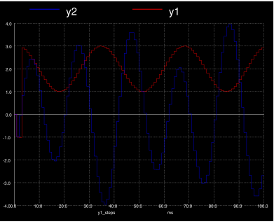
Real matrix gain test.
*
.control
tran 1e-3 1e-1
save all
plot u1 u2 u3
plot y1 y2
.endc
*
* Model inputs
*
v1 1 0 pulse(-1 1 1m 1m 1m 100m 200m)
r1 1 0 1k
v2 2 0 sin(0 1 50)
r2 2 0 1k
v3 3 0 sin(0 1 30 0 0 90)
r3 3 0 1k
*
* Clock signal generation
*
vpulse npulse 0 pulse(0 1 0 1e-6 1e-6 0.5e-3 1e-3)
abridge1 [npulse] [clk] atod
.model atod adc_bridge
*
* Analog voltage to real number conversion
*
a1r 1 clk u1 ator1
.model ator1 ana_to_real(clk_low=0.1 clk_high=0.9 delay=1e-9)
a2r 2 clk u2 ator2
.model ator2 ana_to_real(clk_low=0.1 clk_high=0.9 delay=1e-9)
a3r 3 clk u3 ator3
.model ator3 ana_to_real(clk_low=0.1 clk_high=0.9 delay=1e-9)
*
* Calculate matrix-vector product
*
amtxprod [ u1 u2 u3 ] clk [ y1 y2 ] mtxprod
.model mtxprod real_mtx_gain(g=[ 2 0 1 0 3 -1 ] delay=1e-9)
*
.end
First part of the simulation includes commands which start a transient simulation with a maximum time step of 1ms and plots input, output signals. In the next part, input signals are defined
- \(u_1\) is rectangular pulse,
- \(u_2=sin(2\cdot 50 \cdot \pi t)\)
- \(u_3=cos(2\cdot 30 \cdot \pi t)\)
Clock pulse is 1KHz and generated by supplying a pulse to an analog-to-digital bridge. Input voltages are converted to real data type by ana_to_real blocks. Finally, input is multiplied by gain matrix to obtain \(y_t\).
$$y_t = \begin{bmatrix} 2 & 0 & 1 \\ 0 & 3 & -1 \end{bmatrix}u_t$$
You should visit Ngspice documentation for further information on spice netlist format and parameters.
Simulation result

The matrix vector product and visualization of time domain signals can be implemented in any programming language, besides the tools like MATLAB/Octave, Python's numpy and matplotlib make it very easy for the developer. On the other hand, such an Xspice code-model implementation given in the article lets the developer combine it with various other physical models like, OpAmp, diodes, logical gates and mix DES with continuous time simulations.