Digital control of continuous time systems

Control systems and sampling

It became highly common to implement controllers by using digital signal processing (DSP) units in the control loop applications. Attaching a digital controller to a physical system requires additional components for interfacing the real-life system to the DSP. The signals to be captured from the physical system are continuous in time and value. For example, the voltage measured from a capacitor is a real number value and available at any time instant. However, the same voltage value should be represented in discrete memory blocks of a DSP memory with a finite number of bits. Hence, it should be discretized in time and quantized in value.

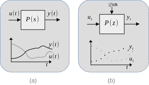
Continuous and discrete time signals — Discrete time signals are obtained from momentary values of continuous time real valued signals quantized into a finite number of bits.

The continuous time real valued signals can be sampled by analog-to-digital converter hardware which is already included in many micro-controller units (MCUs) or can be attached to DSPs as a separate integrated circuit (IC).

System bandwidth

When formulating digital control of an continuous time linear time-invariant (LTI) system, the non-linearity introduced by sampling should be considered. The sampling frequency should be selected as large enough to make the non-linear effects negligible. "Generally, sample rates should be faster than 30 times the bandwidth in order to assure that the digital controller can be made to closely match the performance of the continuous time controller." [1]

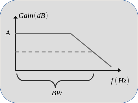
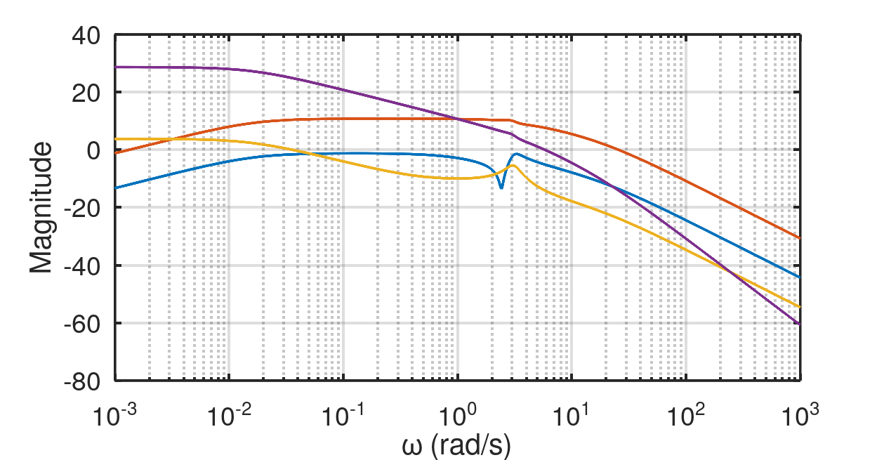
The frequency response plot below shows the definition of bandwidth (BW) graphically. In the frequency response, there is a region where the gain is approximately $A$. The BW is the frequency axis width of this region. Outside of this region gain drops and frequency components in the low gain regions are suppressed by the system.

Sampling and aliasing

The effect of sampling can be described mathematically by using Dirac delta functions. Assume a continuous time signal $y(t)$, the sampled version of $y(t)$ at sampling frequency $F_s$ can be written as

$$y_s(t) = y(t) \sum_{n=-\infty}^{\infty} \delta(t-n/F_s),$$

where $\delta$ is the Dirac delta function. The Fourier transform of $y_s(t)$ gives the frequency response of sampled function.

$$Y_s(f) = Y(f) \ast \sum_{n=-\infty}^{\infty} \delta(f-nF_s),$$

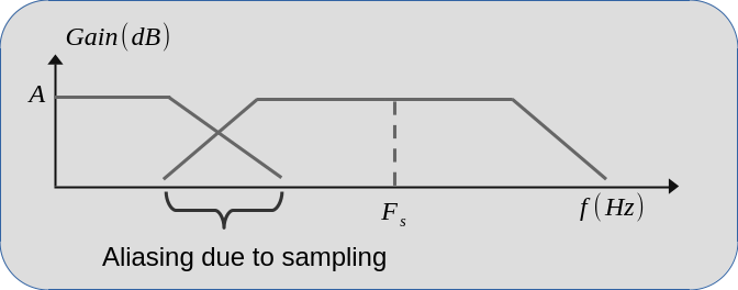
where $Y(f)$ is the Fourier transform of $y(t)$ and $\ast$ denotes the convolution operation. So, $Y_s(f)$ is the sum of repeating $Y(f)$ centered at frequencies $0, F_s, 2F_s, 3F_s, \dots$. This effect is shown in the figure below. As it can be seen sum of overlapped region increases the gain at high frequencies. A controller designed for $Y(f)$ will receive unexpectedly large high frequency signals. It will cause ripples in the output of controller and may cause unstability.

Aliasing caused by sampling — Effect of aliasing due to choosing a small sampling frequency ($F_s$)

Digital control

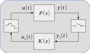
The figure below shows a digital control system where $P(s)$ is the plant (physical system to be controlled) and $y(t)$ is the output (measurement). The output is sampled and digital control rule $K(z)$ calculates control input $u_s(t)$ which is converted to the continuous time signal $u(t)$. In an actual system, the right-most and left-most blocks can be considered as analog-to-digital converter (ADC) and digital-to-analog converter (DAC) correspondingly.

In the equations above, sampled version $y_s(t)$ of $y(t)$ is represented in the frequency domain as

$$Y_s(f) = Y(f) \ast \sum_{n=-\infty}^{\infty} \delta(f-nF_s).$$

In order to simplify, assume that $K(z)$ is a static output feedback gain which is the simplest controller form. Then, $u_s(t)$ becomes

$$u_s(t) = K y_s(t),$$

which leads to

$$U_s(f) = KY_s(f) = K Y(f) \ast \sum_{n=-\infty}^{\infty} \delta(f-nF_s).$$

The effect of DAC block can be represented mathematically as

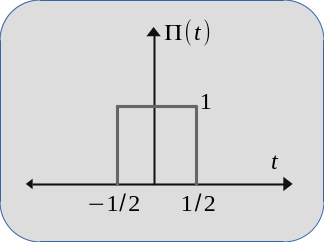
$$u(t) = u_s(t) \ast \Pi(t F_s - 1/2),$$

where $\Pi(t)$ is the rectangular function

$$\Pi(t) = \begin{cases} 0 ~~ \textrm{if} ~~ |t| > 1/2 \\ 1 ~~ \textrm{if} ~~ |t| < 1/2 \\ 1/2 ~~ \textrm{if} ~~ |t| = 1/2 \end{cases}.$$

When the control input $u(t)$ transformed to the frequency domain

$$U(f) = U_s(f) \frac{1}{F_s} \textrm{sinc}\left(\frac{\pi f}{F_s}\right) e^{-j\pi f/F_s}$$

where the sinc function has a bandwidth of $\pi F_s$.

If $F_s$ is chosen a sufficiently large value

$$Y_s(f) \approx Y(f) ~~ \textrm{and} ~~ U(f) \approx U_s(f),$$

$$U(f) \approx K Y(f) \Rightarrow u(t) \approx Ky(t).$$

In other words, the digital control system closely matches the continuous time version when the sampling frequency $F_s$ is chosen sufficiently large.

An example

Let us revisit the aircraft example from a previous article where $P(s)$ is defined by

$$P(s) = C\left(sI-A\right)^{-1}B.$$

The system $P(s)$ is unstable because of the rudder actuator failure in the model [2]. Its effect is mathematically modeled by the entry in system matrix $A_{6,6} = 0.001$. The bandwidth concept is not meaningful for unstable systems, because high frequency input (out of band input) will not be suppressed. As a matter of fact, any input or non-zero initial condition will cause the system output magnitude increase indefinitely as $t \rightarrow \infty$. However, removing the failed rudder actuator from system dynamics and plotting the frequency response will give an idea about the system BW. The frequency response after removing the unstable part is given in the figure below. As it can be seen, it is adequate to choose $10rad/s \approx 3\textrm{Hz}$ as the system BW. So, 100Hz sampling frequency should be enough to approximate a continuous time controller.

The algorithm presented in this thesis [2] is used to calculate a stabilizing static output feedback (SOF) gain. When the sampling frequency is chosen as 100Hz, this implementation of the algorithm returns the gain matrix

$$K_{\textrm{100Hz}} = \begin{bmatrix} 0.1571 & 0.6951 & -1.6636 & 0.827 \\ 0.2387 & -0.0357 & 0.0461 & -0.0374 \end{bmatrix}.$$

When the sampling frequency is chosen 10Hz, the stabilizing SOF gain below is obtained

$$K_{\textrm{10Hz}} = \begin{bmatrix} 0.1069 & 0.2156 & -0.9766 & 0.295 \\ 0.0228 & -0.0057 & 0.012 & -0.0056 \end{bmatrix}.$$

Simulation results

The simulations are implemented in Spice netlist language by using this fork of NGSpice because the original NGSpice does not include some models used in this simulation. The netlist below implements the 100Hz sampling frequency version.

Digital control of continuous time systems
.control
tran 1e-4 0.1e2
options filetype=ascii
plot v(y1) v(y2) v(y3) v(y4)
plot v(u1) v(u2)
.endc
.include "unstable_plane_fb_sum.lib"
.include "unstable_plane_model.lib"
V1 extu1 0 PULSE( 0 0 2u 2u 2u 199 200 )
V2 extu2 0 PULSE( 0 0 2u 2u 2u 199 200 )
*
vpulse npulse 0 pulse(0 1 0 1e-6 1e-6 0.5e-2 1e-2)
abridge1 [npulse] [clk] atod
.model atod adc_bridge
*
aator1 y1 clk y1d ator1
.model ator1 ana_to_real(clk_low=0.1 clk_high=0.9 delay=1e-9)
*
aator2 y2 clk y2d ator2
.model ator2 ana_to_real(clk_low=0.1 clk_high=0.9 delay=1e-9)
*
aator3 y3 clk y3d ator3
.model ator3 ana_to_real(clk_low=0.1 clk_high=0.9 delay=1e-9)
*
aator4 y4 clk y4d ator4
.model ator4 ana_to_real(clk_low=0.1 clk_high=0.9 delay=1e-9)
*
amtxprod [y1d y2d y3d y4d] clk [outd1 outd2] mtxprod
.model mtxprod real_mtx_gain(g=[0.1571 0.6951 -1.6636 0.827 0.2387 -0.0357 0.0461 -0.0374] delay=1e-9)
*
acont1 outd1 out1 rtoa1
.model rtoa1 real_to_v(gain=1.0 transition_time=1e-9)
acont2 outd2 out2 rtoa2
.model rtoa2 real_to_v(gain=1.0 transition_time=1e-9)
*
XLTI2 0 extu1 extu2 out1 out2 u1 u2 unstable_plane_fb_sum
*
XLTI1 0 u1 u2 y1 y2 y3 y4 unstable_plane_model
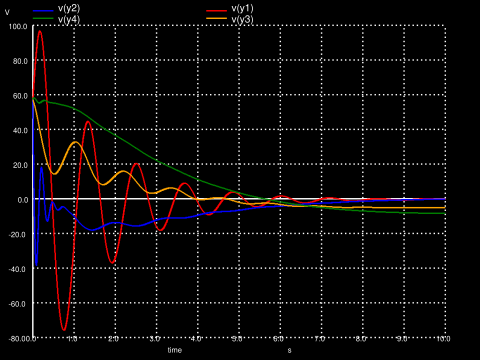
.end

The netlist uses unstable_plane_fb_sum.lib and unstable_plane_model.lib which are discussed in a previous article. They can be downloaded from unstable_plane_fb_sum.lib and unstable_plane_model.lib. The sampling frequency is adjusted by the last two parameters in the line "vpulse npulse 0 pulse(0 1 0 1e-6 1e-6 0.5e-2 1e-2)". The plot below shows the simulation results when the initial condition is

$$x(0) = \left[ 1~~1~~1~~1~~1~~1~~1 \right]^T.$$

The next netlist implements the 10Hz sampling frequency version.

Digital control of continuous time systems
.control
tran 1e-4 0.1e2
options filetype=ascii
plot v(y1) v(y2) v(y3) v(y4)
plot v(u1) v(u2)
.endc
.include "unstable_plane_fb_sum.lib"
.include "unstable_plane_model.lib"
V1 extu1 0 PULSE( 0 0 2u 2u 2u 199 200 )
V2 extu2 0 PULSE( 0 0 2u 2u 2u 199 200 )
*
vpulse npulse 0 pulse(0 1 0 1e-6 1e-6 0.5e-1 1e-1)
abridge1 [npulse] [clk] atod
.model atod adc_bridge
*
aator1 y1 clk y1d ator1
.model ator1 ana_to_real(clk_low=0.1 clk_high=0.9 delay=1e-9)
*
aator2 y2 clk y2d ator2
.model ator2 ana_to_real(clk_low=0.1 clk_high=0.9 delay=1e-9)
*
aator3 y3 clk y3d ator3
.model ator3 ana_to_real(clk_low=0.1 clk_high=0.9 delay=1e-9)
*
aator4 y4 clk y4d ator4
.model ator4 ana_to_real(clk_low=0.1 clk_high=0.9 delay=1e-9)
*
amtxprod [y1d y2d y3d y4d] clk [outd1 outd2] mtxprod
.model mtxprod real_mtx_gain(g=[0.1069  0.2156 -0.9766  0.295 0.0228 -0.0057  0.012  -0.0056] delay=1e-9)
*
acont1 outd1 out1 rtoa1
.model rtoa1 real_to_v(gain=1.0 transition_time=1e-9)
acont2 outd2 out2 rtoa2
.model rtoa2 real_to_v(gain=1.0 transition_time=1e-9)
*
XLTI2 0 extu1 extu2 out1 out2 u1 u2 unstable_plane_fb_sum
*
XLTI1 0 u1 u2 y1 y2 y3 y4 unstable_plane_model
.end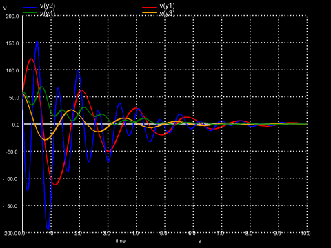

Conclusion

When the low sampling frequency result is compared to high frequency one, it can be observed that low sampling rate leads to extensive high frequency effects on the output. One can see larger overshoots and large oscillations which are caused by the non-linear effect due to aliasing. These effects are not handled by the SOF controller. Although the output seems stable, it is not guaranteed to be stable for all initial conditions. The output magnitude may increase indefinitely by time when $x_0$ is started from an other point in the state space.