Systems modeling and control theory are intellectual products resulting from the human ambition on understanding and taming the natural phenomena for exploiting its use value. Unmanageable systems, in other words unstable systems, are generally considered to be useless. In order to make it useful, the source of unstability should be discovered and an appropriate stabilizing control technique should be implemented.
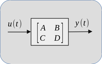
For the continuous time linear time-invariant (LTI) system which are defined by the state space equations
$$\dot{x}=Ax+Bu ~~~~~~~~~~ (1)$$
$$y=Cx+Du,$$
where
- $x \in \mathbb{R}^n$ is the n-dimensional vector of state variables
- $u \in \mathbb{R}^m$ is the m-dimensional vector of input
- $y \in \mathbb{R}^r$ is the r-dimensional vector of output
- $A \in \mathbb{R}^{n \times n}$ n-by-n state matrix
- $B \in \mathbb{R}^{n \times m}$ n-by-m input matrix
- $C \in \mathbb{R}^{r \times n}$ r-by-n output matrix
- $D \in \mathbb{R}^{r \times m}$ r-by-m input-to-output matrix,
solution of the linear ordinary differential equation (ODE) above for given $u(t)$ and $x(0)$ determines the trajectory that the system will follow. In order to simplify the problem, let us consider the case where $u(t) = 0$ for all $t$ from $t=0$ to the final time $t=t_f$. By this, the equations are reduced to
$$\dot{x}=Ax, ~~~ y = Cx.$$
In general, the solution of $i$th entry in the output vector $y$ is
$$y_i(t)=\sum_{k=1}^{n} e^{\zeta_k t} \left(M_k \cos(\omega_k t) + N_k \sin(\omega_k t) \right),$$
where $M_k,N_k,\zeta_k$ are constants. For a stable (exponentially stable) system,
$$ \zeta_k < 0, ~~ \textrm{for all} ~ k $$
must be satisfied, so the integral
$$ \int_{0}^{\infty}|y_i(t)| dt $$
will be bounded for any initial $y(0)=Cx(0)$. This will make $y(t)$ bounded for any bounded input $u(t)$. The coefficients $\zeta_k$ are determined by the eigenvalues of system matrix $A$ and the sign of $\zeta$ depends on the sign of real part of $A$'s eigenvalues. More precisely, the real parts of all eigenvalues of $A$ must be negative. Luckly, the eigenvalues can be placed to have negative real parts by an appropriate feedback controller if the system is stabilizable.
All control problem should cover the stabilization problem, because one can not reach the control goals like
- steering the system's output in a desired way: $ \min \|y_{desired}(t)-y(t)\| $
- minimizing the required input energy: $ \min \| u(t) \|^2 $
- drive the system's output to a desired value in a minimum amount of time: $ \min y_{t_f}, ~ \textrm{given} ~ y(t_f) = y_{t_f} $
- etc.
with an unstable (unusable) system.
Example
Let us consider the unstable aircraft example from a previous article.
$$ -1.000,-3.615,-0.423+3.063i,-0.422-3.063i,-0.0163,-20.02,0.001 $$
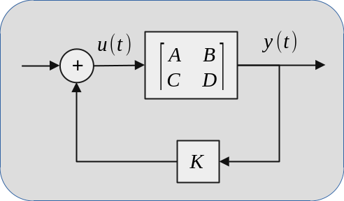
As it can be seen, the last eigenvalue has a real part greater than zero. This causes one of the $\zeta$ values to be greater than zero which makes the system unstable. However, all eigenvalues can be made stable by a static output feedback (SOF) controller. This requires measuring the system output, multiplying it by a constant matrix and feeding the result to the system input.
The open loop system is defined by Equation 1 above. After multiplying system output $y$ by the SOF gain $K$ and choosing input
$$ u = Ky $$
Equation 1 becomes
$$ \dot{x} = Ax+Bu = Ax+BKy = Ax+BKCx $$
$$ \dot{x} = (A+BKC)x, $$
where all eigenvalues of $A+BKC$ has negative real parts.
When $K$ is chosen as given in this article, the eigenvalues of closed loop system becomes.
$$ -11.2497+22.8353i,-11.2497-22.8353i,-0.7791+5.348i,-0.7791-5.348i,-1.1694,-0.3178,-0.1311 $$
where all have negative real parts. Meaning that, the closed loop system is stable.
The static feedback gain $K$ introduces a self-regulation behavior that eliminates the unstability of the original system. From this point on, the designer can continue working on the actual control goal with the advantage of dealing with an internally stable system.